Linear Deconvolution

Posted on 2016-06-09 | In Digital Signal Processing |

Deconvolution problem is a subset of inversion, in which observed data is deconvolved to reconstruct the model given the blurring function or source wavelet. Items of inversion including “resolution”, “error”, “regularization”, et. al also apply to deconvolution. Besides, deconvolution always associates transformation between time domain and frequency domain. Thus, principles inherited from digital singal processing apply to deconvolution. In other words, deconvolution is very complex, though massive codes and programs could output a time series in a blink of eye given no matter what kind of data input. Without comprehension of deconvolution and inversion, programs could be misused to provide wrong results. This blog attempts to theories and implementations of deconvolution.

利用总控Makefile一次性编译所有子程序包

Posted on 2016-06-09 | In Programming |

当一个大的项目由很多子程序组成，而每一个子程序包都有自己独立的Makefile，这时候就需要一个总控Makefile来一次性完成所有的编译工作。以下给出了一个例子，以说明如何构建总控Makefile。

怎么在linux下压缩和解压文件

Posted on 2016-06-09 | In Linux工具及配置 |

此文是写给呆萌女朋友的。

Linux终端美化

Posted on 2016-06-08 | In Linux工具及配置 |

不知道你是不是受够了Linux终端的丑陋。黑色衬底配上刺眼的颜色和奇怪的字体，是默认Linux的终端外观。如果你长期需要在Linux下作业，那么一个养眼的终端带来的将是身心愉悦，效率翻倍，毕竟这是一个凡事看脸的时代，颜即正义。

使用github和hexo搭建静态博客

Posted on 2016-06-08 | In Hexo |

Hello World

Ray Tracing (2) Pseudo Bending Method

Posted on 2015-10-26 | In Seismic Tomography |

This post is about the pseudo bending method provided by Junho Um and Clifford Thurber. Test and codes are provided.

Intro

The key point of bending method is ray path calibration, which could be calculated according to $\eqref{rt1}$.

$\begin{eqnarray} \frac{d^2x_i}{ds^2} = \frac{1}{c} ( -\frac{dc}{dx_i} + \frac{dc}{ds}\frac{dx_i}{ds} ) \label{rt1}\\ % T = \int_s \frac{1}{c}ds \label{rt2} \end{eqnarray}$

In $\eqref{rt1}$, the left side is the ray path curvature, while the right side states the velocity gradient component normal to the ray path. This ray path curvature direction gives the calibration direction for each points:

$\begin{eqnarray} \vec{n} = \nabla c - \frac{\vec{dx}}{|\vec{dx}|^2}\nabla c \cdot \vec{dx} \label{cur} \end{eqnarray}$

The amount of calibration $R_c$ is obtained by minimizing the travel time.

Computation

Discretize the seismic ray and analyze a segment of it:

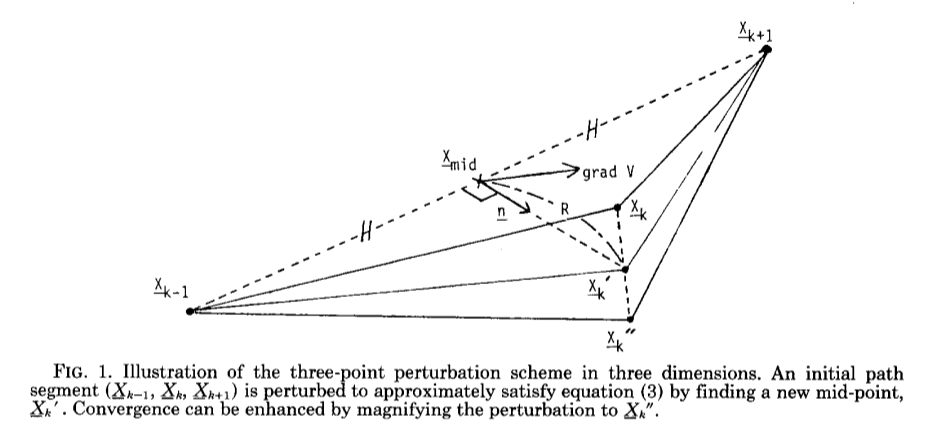
The travel time for discretized ray path is:

$\begin{eqnarray} T = \sum_{k=2}^{N} |\vec{X_k} - \vec{X_{k-1}}| \frac{c_k+c_{k-1}}{2} \end{eqnarray}$

According to $\eqref{cur}$, the curvature direction for segment ($X{k-1}X{k+1}$) should be:

$\begin{eqnarray} \vec{n} & = & \nabla c - \frac{\vec{X}_{k+1}- \vec{X}_{k-1}} {|\vec{X}_{k+1}- \vec{X}_{k-1}|^2}\nabla c \cdot (\vec{X}_{k+1}- \vec{X}_{k-1}) \label{e1} \end{eqnarray}$

After having the curvature direction, a initial point is required. The mid-point is choosed, and the ideal point is $X_k’$.

Calibration amount is obtained by minimizing the travel-time of segment $X{k-1} \rightarrow X_k’ \rightarrow X{k+1}$.

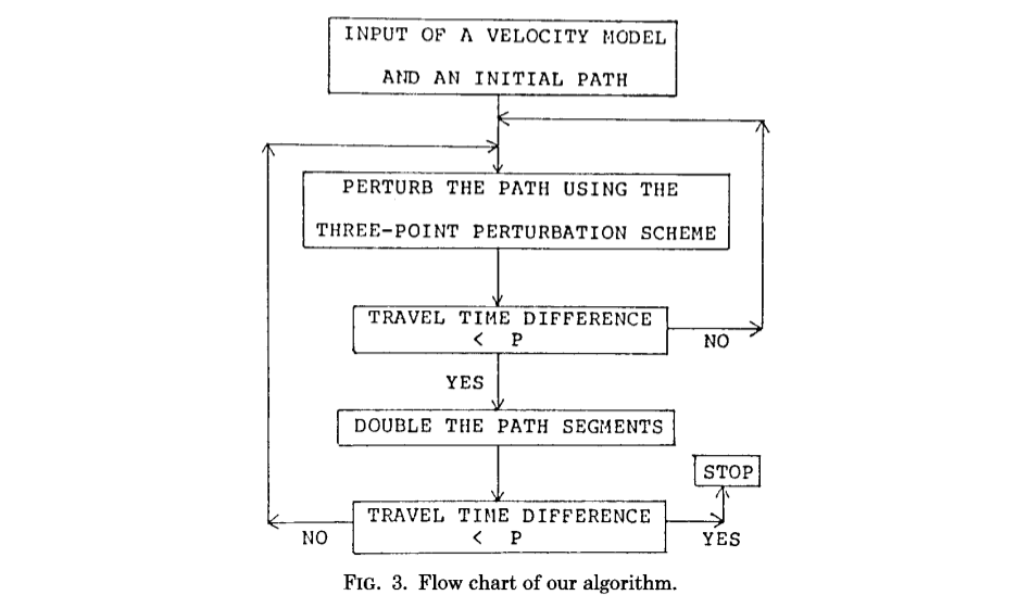
$\begin{eqnarray} R_c & = & -\frac{c_a c_{mid} + 1}{4c_a \vec{n}_0 \cdot \nabla c_{mid}} + \sqrt{ \Big( \frac{c_a c_{mid}+1}{4c_a \vec{n}_0 \cdot \nabla c_mid} \Big) + \frac{ |\vec{X}_{k+1} - \vec{X}_{mid}|^2}{ 2c_a c_{mid} } } \label{e2} \\ c_a & = & \frac{1}{2} \Big( \frac{1}{c_{k-1}} + \frac{1}{c_{k+1}} \Big) \\ \vec{n}_0 & = & \frac{ \vec{n} }{|\vec{n}|} \end{eqnarray}$

For each points of the seismic ray, apply $\eqref{e1}$ and $\eqref{e2}$ to acquire the new point. Repeat this procedure until the traveltime converges.

Moreover, more ray path control points are require for traveltime convergence. Um and Thurber provides a flow chart:

Codes & Test

1D constant gradient model

For one-dimensional constant velocity gradient model, the analytic ray path is an arc, the red line presented bellow. Ray paths of iteration are presented in black lines, which finally converge to the analytic ray path.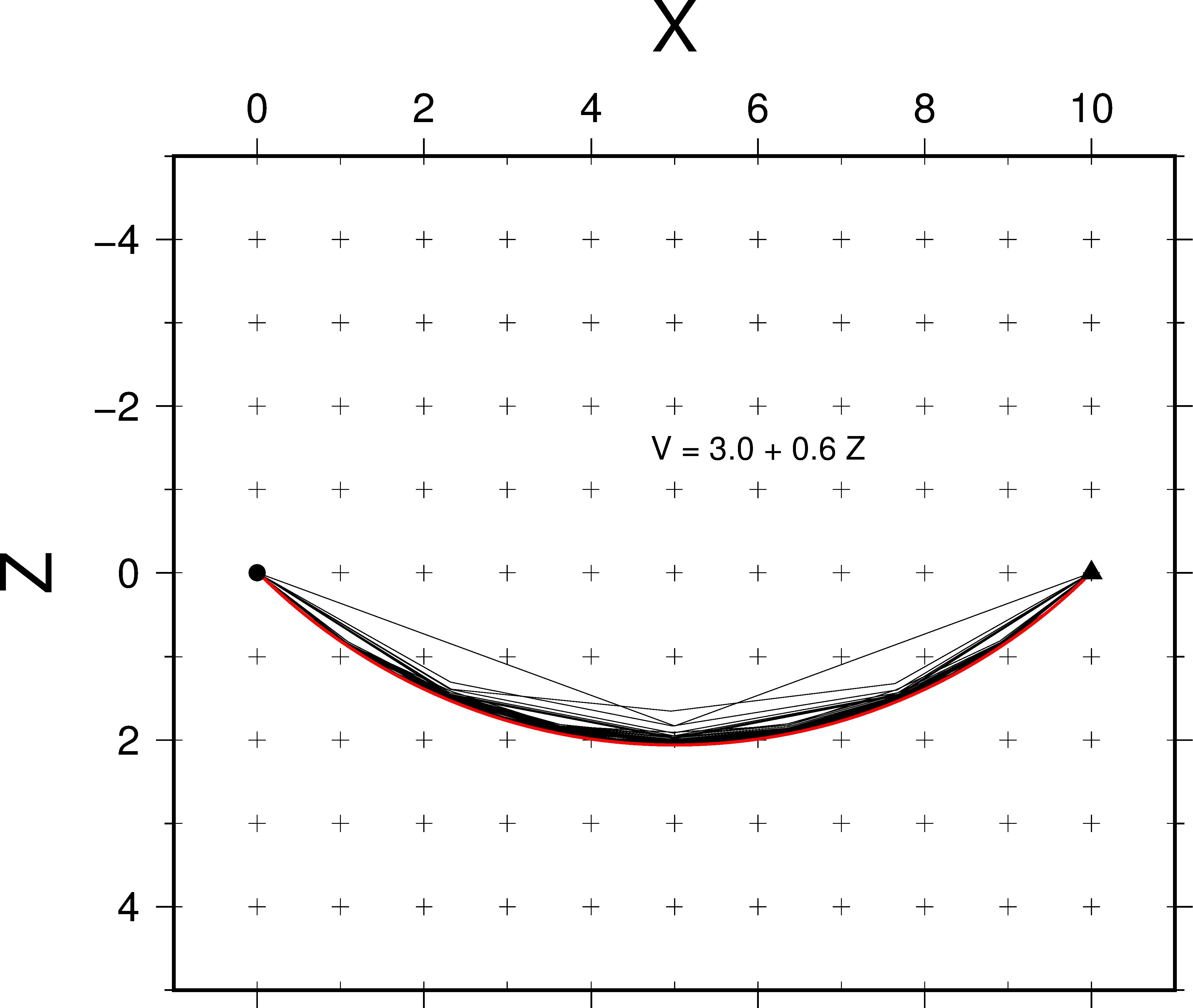

Codes

codes

bash> make
bash> ./main > path.dat
bash> ./plot.sh # "path.jpg" is the image of raypath
bash>

Reference

Um, J.,C.H. Thurber, A fast algorithm for two-point seismic ray tracing. Bull Seismol Soc Am.Bulletin of the Seismological Society of America, 1987. 77(3).

Ray Tracing (1) Derivation

Posted on 2015-10-26 | In Seismic Tomography |

Give acoustic wave equation $\eqref{acoustic_wave}$, consider the harmonic solution $\eqref{harmonic_sol}$, where $c(x_i)$ is the velocity, $T(x_i)$ the travel time.

$\begin{eqnarray} \nabla^2\phi & = & \frac{1}{c^2(x_i)}\phi \label{acoustic_wave} \end{eqnarray}$ $\begin{eqnarray} \phi(x_i) & = & \Phi(x_i)exp[-i\omega(t-T(x_i))] \label{harmonic_sol} \end{eqnarray}$

Applying the high frequency approximation, eikonal equation$\eqref{eikonal_eq}$ and transport equation $\eqref{transport_eq}$ are derived. $\textbf{p}$, the slowness vector, which is perpendicular to the wavefront, the contour of travel time $T$, declares the propagation direction of waves.

$\begin{cases} \begin{eqnarray} & & p_ip_i = \frac{1}{c^2(x_i)} \label{eikonal_eq} \\ & & p_i = (\nabla T)_i \\ & & 2 \nabla \Phi \cdot \nabla T+ \Phi \nabla^2T = 0 \label{transport_eq} \end{eqnarray} \end{cases}$

Build Hamilton equation for eikonal equation, where $s$ declares the ray path.

$\begin{cases} \begin{eqnarray} H(x_i, p_i) & = & (p_ip_i)^{1/2} - c^{-1}(x_i) \label{hamilton_eq} \\ \frac{dx_i}{ds} & = & \frac{\partial H}{\partial p_i} \\ \frac{dp_i}{ds} & = & \frac{\partial H}{\partial x_i} \\ \frac{dT}{d} & = & p_i \frac{\partial H}{\partial p_i} \end{eqnarray} \end{cases}$

Derivation ends here. In the right side of $\eqref{rt1}$, $\frac{dc}{dx_i}$ is the velocity gradient, $\frac{dc}{ds}\frac{dx_i}{ds}$ the projection of velocity gradient along ray path. In the left side, $\frac{d^2x_i}{ds^2}$ declares the curvature direction of ray path. Thus, the direction change of ray path can be calculated given the velocity gradient and ray path direction. Or, given a initial ray path direction, we could derive each segments of ray path.

$\begin{eqnarray} \frac{d^2x_i}{ds^2} = \frac{1}{c} ( -\frac{dc}{dx_i} + \frac{dc}{ds}\frac{dx_i}{ds} ) \label{rt1}\\ % T = \int_s \frac{1}{c}ds \label{rt2} \end{eqnarray}$

However, the boundary condition problem, the two-point ray tracing problem, but not initial condition problem is much more prevalent. It could be solved using iteration, and the ray path is calibrated in each step according to $\eqref{rt1}$. This is bending method.

Reference
Cerveny, V.,M.G. Brown, Seismic Ray Theory. Applied Mechanics Reviews, 2002. 55(6): p.14.

Const Reference in Function Parameters

Posted on 2015-05-21 | In Programming |

This post presents tips of using const reference in functions. Examples are presented for wrong using.