Finite Difference of Staggered Grid (2)

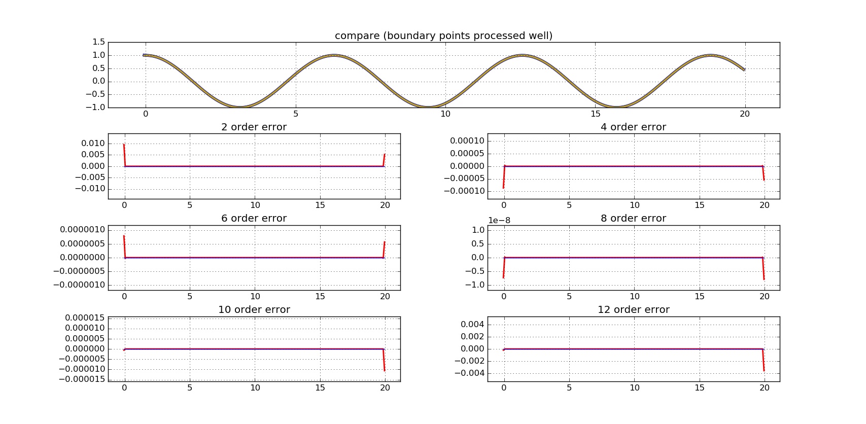
This post presents the asymmetric finite-difference scheme build in staggered grid. This asymmetric scheme works well for processing boundary points.

• $f’(x)$ in 2nd order accuracy
  • point 0
• $f’(x)$ in 2Nth order accuracy
  • point 0
  • point k $(k=0,1,2,3…,N-1)$
• Conclusion
• Examples

$f’(x)$ in 2nd order accuracy

point 0

To calculate the first order derivates in the $\color{blue}{blue}$ grid points, values in $\color{red}{red}$ points are expanded.

$$\begin{eqnarray} f(x+\frac{\delta}{2}) & = & f(x) + \frac{\delta}{2} f'(x) + \frac{\delta^2}{2^2 2!}f''(x) + O(\delta^3) \\ %+\frac{\delta^N}{2^N N!}f^{(N)}(x) %+ O(\delta^{N+1}) \\ f(x+\frac{3\delta}{2}) & = & f(x) + \frac{3\delta}{2} f'(x) + \frac{3^2\delta^2}{2^2 2!}f''(x) + O(\delta^3) \\ %+ ... %+ \frac{3^N\delta^N}{2^N N!}f^{(N)}(x) %+ O(\delta^{N+1}) \\ f(x+\frac{5\delta}{2}) & = & f(x) + \frac{5\delta}{2} f'(x) + \frac{5^2\delta^2}{2^2 2!}f''(x) + O(\delta^3) \\ %+ ... %+ \frac{5^N\delta^N}{2^N N!}f^{(N)}(x) %+ O(\delta^{N+1}) \end{eqnarray}$$

thus, $f’(x)$ are:

$$\begin{eqnarray} f'(x) & = & \frac{2 f(x+\frac{\delta}{2}) }{\delta} -\frac{2 f(x)}{\delta} - \frac{\delta}{2 2!}f''(x) + O(\delta^3) \\ %- ... %-\frac{\delta^{N-1}}{2^{N-1} N!}f^{(N)}(x) %+ O(\delta^{N}) \\ f'(x) & = & \frac{2 f(x+\frac{3\delta}{2}) }{3\delta} -\frac{2 f(x) }{3\delta} - \frac{3\delta }{2 2!}f''(x) + O(\delta^3) \\ %- ... %- \frac{3^{N-1}\delta^{N-1}}{2^{N-1} N!}f^{(N)}(x) %+ O(\delta^{N}) \\ f'(x) & = & \frac{2 f(x+\frac{5\delta}{2}) }{5\delta} -\frac{2 f(x) }{5\delta} - \frac{5\delta }{2 2!}f''(x) + O(\delta^3) \\ %- ... %- \frac{5^{N-1}\delta^{N-1}}{2^{N-1} N!}f^{(N)}(x) %+ O(\delta^{N}) \end{eqnarray}$$

add these $f’(x)$ proportionally:

$$\begin{equation} \begin{aligned} f'(x) = & \frac{2}{\delta} \left[ C^2_{00} f(x + \frac{\delta}{2}) + C^2_{01}\frac{1}{3} f(x + \frac{3\delta}{2} )+ C^2_{02}\frac{1}{5} f(x + \frac{5\delta}{2} ) \right]\\ & -\frac{2}{\delta} \left[ C^2_{00}+ \frac{1}{3}C^2_{01}+ \frac{1}{5}C^2_{02} \right] f(x) - \frac{\delta}{2 2!} \left[ C^2_{00}+ 3C^2_{01}+ 5C^2_{02} \right]f''(x) + O(\delta^3) \end{aligned} \end{equation}$$

In order to have second order accuracy, $C^2_{0j}$ must satisfy the equation of:

$$\begin{equation} \begin{cases} C^2_{00} + C^2_{01} + C^2_{02} = 1\\ C^2_{00} + \frac{1}{3}C^2_{01} + \frac{1}{5}C^2_{02} = 0\\ C^2_{00} + 3C^2_{01} + 5C^2_{02} = 0\\ \end{cases} \Rightarrow \begin{cases} C^2_{00} = -1 \\ C^2_{01} = \frac{9}{2} \\ C^2_{02} = -\frac{5}{2} \end{cases} \end{equation}$$

$f’(x)$ in 2Nth order accuracy

point 0

$$\begin{eqnarray} f(x+\frac{\delta}{2}) & = & f(x) + \frac{\delta}{2} f'(x) + \frac{\delta^2}{2^2 2!}f''(x) + ... +\frac{\delta^{2N}}{2^{2N} (2N)!}f^{(2N)}(x) + O(\delta^{2N+1}) \\ f(x+\frac{3\delta}{2}) & = & f(x) + \frac{3\delta}{2} f'(x) + \frac{3^2\delta^2}{2^2 2!}f''(x) + ... + \frac{3^{2N}\delta^{2N}}{2^{2N} {2N}!}f^{(2N)}(x) + O(\delta^{2N+1})\\ &...&\\ f(x+\frac{l\delta}{2}) & = & f(x) + \frac{l\delta}{2}f'(x) + \frac{l^2\delta^2}{2^2 2!}f''(x) + ... + \frac{l^{2N}\delta^{2N}}{2^{2N} (2N)!}f^{(2N)}(x) + O(\delta^{2N+1}) \end{eqnarray}$$

thus, $f’(x)$ are:

$$\begin{eqnarray} f'(x) & = & \frac{2 f(x+\frac{\delta}{2}) }{\delta} -\frac{2 f(x)}{\delta} - \frac{\delta}{2 2!}f''(x) - ... -\frac{\delta^{2N-1}}{2^{2N-1} (2N)!}f^{(2N)}(x) + O(\delta^{2N}) \\ f'(x) & = & \frac{2 f(x+\frac{3\delta}{2}) }{3\delta} -\frac{2 f(x) }{3\delta} - \frac{3\delta }{2 2!}f''(x) - ... - \frac{3^{2N-1}\delta^{2N-1}}{2^{2N-1} (2N)!}f^{(2N)}(x) + O(\delta^{2N}) \\ &...&\\ f'(x) & = & \frac{2 f(x+\frac{l\delta}{2}) }{l\delta} -\frac{2 f(x) }{l\delta} - \frac{l\delta}{2 2!}f''(x) - ... - \frac{l^{2N-1}\delta^{2N-1}}{2^{2N-1} (2N)!}f^{(2N)}(x) + O(\delta^{2N}) \\ \color{red}{(l=1,3,5,7,9...)} \end{eqnarray}$$

add these $f’(x)$ proportionally:

$$\begin{equation} \begin{aligned} f'(x) = & \frac{2}{\delta} \sum \limits_l \left[ f(x + \frac{l\delta}{2}) C^{2N}_{0(\frac{l-1}{2})}\frac{1}{l} \right]\\ &-\frac{2}{\delta}f(x) \sum \limits_l \left[ C^{2i}_{0(\frac{l-1}{2})} \frac{1}{l} \right] -\frac{\delta}{2 2!} f''(x) \sum \limits_l \left[ C^{2i}_{0(\frac{l-1}{2})} l \right]\\ & -... -\frac{\delta^{2N-1}}{2^{2N-1} (2N)!} f^{2N}(x) \sum \limits_l \left[ C^{2N}_{0(\frac{l-1}{2})} l^{2N-1} \right] +O(\delta^{2N})\\ (l=1,3,5,7,9...) \end{aligned} \end{equation}$$

To have 2Nth order accuracy, , $C^{2N}_{0j}$ must satisfy the equation:

$$\begin{eqnarray} \begin{bmatrix} 1 & 1 & 1 & ... & 1 \\ 1 & \frac{1}{3} & \frac{1}{5}& ... & \frac{1}{4N+1} \\ 1 & 3 & 5 & ... & 4N+1 \\ 1 & 3^2 & 5^2 & ... & (4N+1)^2 \\ ...\\ 1 & 3^{2N-1} & 5^{2N-1} & ... & (4N+1)^{2N-1} \\ \end{bmatrix} \begin{bmatrix} C^{2N}_{00} \\ C^{2N}_{01} \\ C^{2N}_{02} \\ C^{2N}_{03} \\ ...\\ C^{2N}_{0(2N)} \\ \end{bmatrix} = \begin{bmatrix} 1\\ 0\\ 0\\ 0\\ ...\\ 0\\ \end{bmatrix} \end{eqnarray}$$

point k $(k=0,1,2,3…,N-1)$

$$\begin{eqnarray} f(x+\frac{(1-2k)\delta}{2}) & = & f(x) +\frac{(1-2k)\delta}{2} f'(x) + \frac{(1-2k)^2\delta^2}{2^22!}f''(x) +... + \frac{(1-2k)^{2N}\delta^{2N}}{2^{2N}(2N)!}f^{(2N)}(x) + O(2N+1) \\ ... \\ f(x-\frac{\delta}{2}) & = & f(x) - \frac{\delta}{2}f'(x) + \frac{\delta^2}{2^22!}f''(x) + ... + \frac{(-1)^{2N}\delta^{2N}}{2^{2N} (2N)!}f^{(2N)}(x) + O(\delta^{2N+1}) \\ f(x+\frac{\delta}{2}) & = & f(x) + \frac{\delta}{2} f'(x) + \frac{\delta^2}{2^2 2!}f''(x) + ... +\frac{\delta^{2N}}{2^{2N} (2N)!}f^{(2N)}(x) + O(\delta^{2N+1}) \\ f(x+\frac{3\delta}{2}) & = & f(x) + \frac{3\delta}{2} f'(x) + \frac{3^2\delta^2}{2^2 2!}f''(x) + ... + \frac{3^{2N}\delta^{2N}}{2^{2N} (2N)!}f^{(2N)}(x) + O(\delta^{2N+1})\\ &...&\\ f(x+\frac{l\delta}{2}) & = & f(x) + \frac{l\delta}{2}f'(x) + \frac{l^2\delta^2}{2^2 2!}f''(x) + ... + \frac{l^{2N}\delta^{2N}}{2^{2N} (2N)!}f^{(2N)}(x) + O(\delta^{2N+1}) \end{eqnarray}$$

thus, $f’(x)$ are:

$$\begin{eqnarray} f'(x) & = & \frac{2}{(1-2k)\delta} f(x+\frac{(1-2k)\delta}{2}) - \frac{2}{(1-2k)\delta} f(x) - \frac{(1-2k)\delta}{2 2!}f''(x) - ... -\frac{(1-2k)^{2N-1}\delta^{2N-1}}{2^{2N-1} (2N)!}f^{(2N)}(x) + O(\delta^{2N}) \\ \\ ... \\ f'(x) & = & \frac{-2}{\delta} f(x-\frac{\delta}{2}) +\frac{2}{\delta} f(x) + \frac{\delta^2}{22!}f''(x) + ... + \frac{(-1)^{2N-1}\delta^{2N-1}}{2^{2N-1} (2N)!}f^{(2N)}(x) + O(\delta^{2N}) \\ f'(x) & = & \frac{2}{\delta} f(x+\frac{\delta}{2}) - \frac{2}{\delta} f(x) - \frac{\delta}{2 2!}f''(x) - ... -\frac{\delta^{2N-1}}{2^{2N-1} (2N)!}f^{(2N)}(x) + O(\delta^{2N}) \\ f'(x) & = & \frac{2}{3\delta} f(x+\frac{3\delta}{2}) -\frac{2}{3\delta}f(x) - \frac{3\delta}{2 2!}f''(x) - ... - \frac{3^{2N-1}\delta^{2N-1}}{2^{2N-1} (2N)!}f^{(2N)}(x) + O(\delta^{2N})\\ &...&\\ f'(x) & = & \frac{2}{l\delta} f(x+\frac{l\delta}{2}) -\frac{2}{l\delta} f(x) - \frac{l\delta}{2 2!}f''(x) - ... - \frac{l^{2N-1}\delta^{2N-1}}{2^{2N-1} (2N)!}f^{(2N)}(x) + O(\delta^{2N}) \end{eqnarray}$$

add these $f’(x)$ proportionally:

$$\begin{equation} \begin{aligned} f'(x) = & \frac{2}{\delta} \sum \limits_l \left[ f( x+ \frac{ l\delta}{2} )C^{2N}_{k(\frac{l-1}{2})} \frac{1}{l} \right] \\ &-\frac{2}{\delta}f(x) \sum \limits_l \frac{1}{l} C^{2N}_{k(\frac{l-1}{2})} -\frac{\delta}{22!}f''(x) \sum \limits_l{l} C^{2N}_{k(\frac{l-1}{2})} -\frac{\delta^2}{2^23!}f^{(3)}(x) \sum \limits_l{l^2}C^{2N}_{k(\frac{l-1}{2})} \\ &-\frac{\delta^3}{2^34!}f^{(4)}(x) \sum \limits_l{l^3}C^{2N}_{k(\frac{l-1}{2})} -... -\frac{\delta^{2N-1}}{2^{2N-1}(2N)!}f^{(2N)}(x) \sum \limits_l{l^{2N-1}}C^{2N}_{k(\frac{l-1}{2})} +O({\delta^{2N}}) \\ &(l = 1-2k, 3-2k,...,-1,1,...) \end{aligned} \end{equation}$$

to have 2Nth order accuracy: $C^{2N}_{kj}$ must satisfy equation:

$$\begin{equation} \begin{bmatrix} 1 & 1 & 1 & ... & 1 \\ \frac{1}{1-2k} & \frac{1}{3-2k} & \frac{1}{5-2k} & ... & \frac{1}{4N-2k+1} \\ 1-2k & 3-2k & 5-2k & ... & 4N-2k+1 \\ (1-2k)^2 & (3-2k)^2 & (5-2k)^2 & ... & (4N-2k+1)^2 \\ ...\\ (1-2k)^{2N-1} & (3-2k)^{2N-1} & (5-2k)^{2N-1} & ... & (4N-2k+1)^{2N-1} \end{bmatrix} \begin{bmatrix} C^{2N}_{k (-k) } \\ C^{2N}_{k (-k+1) } \\ C^{2N}_{k (-k+2) } \\ C^{2N}_{k (-k+3) } \\ ...\\ C^{2N}_{k (2N-k)} \end{bmatrix} = \begin{bmatrix} 1\\ 0\\ 0\\ 0\\ ...\\ 0\\ \end{bmatrix} \label{LA} \end{equation}$$

Conclusion

For 2Nth order accuracy, for point k in the boundary region, value of $f’(x)$ is:

$$\begin{equation} f'(x) = \frac{2}{l\delta} \sum \limits_l \left[ f( x+ \frac{l\delta}{2} )C^{2N}_{k(\frac{l-1}{2})} \right] \\ (l=1-2k,3-2k,...,-1,1,...,4N-2k+1) \end{equation}$$

while $C^{2N}_{kj}$ is solution of equation $\eqref{LA}$.

Or, in the form of:

$$\begin{equation} \begin{cases} f'(x) = \frac{1}{\delta} \sum \limits_l \left[ f( x+ \frac{l\delta}{2} )c^{2N}_{k(\frac{l-1}{2})} \right] \\ c^{2N}_{k(\frac{l-1}{2})} = \frac{2}{l}C^{2N}_{k(\frac{l-1}{2})} \\ (l=1-2k,3-2k,...,-1,1,...,4N-2k+1) \end{cases} \end{equation}$$

Examples

FD scheme corresponding to accuracy orders of 2,4,6,8,10,12 are implemented to $f(x)=sin(x)$, their FD results are ploted versus theoretical first order derivative of $f’(x)=cos(x)$, as well as their error.