Finite Difference of Staggered Grid (1)

This post presents the central finite difference(FD) system build in stagger grid. Symmetric scheme are derived and examples are presented.

• Taylor expansion
• First order derivatives
• Conclusion
• Examples

Taylor expansion

As always, we start the derivation from taylor expansion. For the $\color{red}{red}$ points in the below staggerd point, function value here have the form of taylor series expanded in the $\color{blue}{blue}$ point. This kind of stagger grid scheme is widely used in modeling.

$$\begin{eqnarray} f\left(x-\frac{i\delta}{2}\right) & = & f(x) - \frac{i\delta}{2}f'(x) + \frac{i^2\delta^2}{2^22!}f''(x) - \frac{i^3\delta^3}{2^33!}f^{(3)}(x) %+ \frac{i^4\delta^4}{2^44!}f^{(4)}(x) + ... + \frac{i^{2N}\delta^{2N}}{2^{2N}(2N)!}f^{(2N)}(x) + O(\delta^{2N+1}) \\ & ... &\\ f\left(x-\frac{\delta}{2}\right) & = & f(x) - \frac{\delta}{2}f'(x) + \frac{\delta^2}{2^22!}f''(x) - \frac{\delta^3}{2^33!}f^{(3)}(x) %+ \frac{\delta^4}{2^44!}f^{(4)}(x) + ... + \frac{\delta^{2N}}{2^{2N}(2N)!}f^{(2N)}(x) + O(\delta^{2N+1}) \\ f\left(x+\frac{\delta}{2}\right) & = & f(x) + \frac{\delta}{2}f'(x) + \frac{\delta^2}{2^22!}f''(x) + \frac{\delta^3}{2^33!}f^{(3)}(x) %+ \frac{\delta^4}{2^44!}f^{(4)}(x) + ... + \frac{\delta^{2N}}{2^{2N}(2N)!}f^{(2N)}(x) + O(\delta^{2N+1}) \\ & ... &\\ f\left(x+\frac{i\delta}{2}\right) & = & f(x) + \frac{i\delta}{2}f'(x) + \frac{i^2\delta^2}{2^22!}f''(x) + \frac{i^3\delta^3}{2^33!}f^{(3)}(x) %+ \frac{i^4\delta^4}{2^44!}f^{(4)}(x) + ... + \frac{i^{2N}\delta^{2N}}{2^{2N}(2N)!}f^{(2N)}(x) + O(\delta^{2N+1}) \\ \color{red}{\left(i =1,3,5,7,9...\right)} \\ \end{eqnarray}$$

First order derivatives

$$\begin{eqnarray} \frac{f\left(x+\frac{\delta}{2}\right) - f\left(x-\frac{\delta}{2}\right)}{2} & = & \frac{\delta}{2}f'(x) + \frac{\delta^3}{2^33!}f^{(3)}(x) + ... + \frac{\delta^{2N-1}}{2^{2N-1}(2N-1)!}f^{(2N-1)}(x) + O(\delta^{2N+1}) \\ &...&\\ \frac{ f\left(x+\frac{i\delta}{2}\right) - f\left(x-\frac{i\delta}{2}\right) }{2} & = & \frac{i\delta}{2}f'(x) + \frac{i^3\delta^3}{2^33!}f^{(3)}(x) + ... + \frac{i^{2N-1}\delta^{2N-1}}{2^{2N-1}(2N-1)!}f^{(2N-1)}(x) + O(\delta^{2N+1}) \\ \color{red}{\left(i=1,3,5,7,9...\right)} \\ \end{eqnarray}$$

or in the forms of:

$$\begin{eqnarray} f'(x) & = & \frac{f\left(x+\frac{\delta}{2}\right) - f\left(x-\frac{\delta}{2}\right)}{\delta} - \frac{\delta^2}{2^23!}f^{(3)}(x) - ... - \frac{\delta^{2N-2}}{2^{2N-2}(2N-1)!}f^{(2N-1)}(x) + O(\delta^{2N}) \\ &...&\\ f'(x) & = & \frac{ f\left(x+\frac{i\delta}{2}\right) - f\left(x-\frac{i\delta}{2}\right) }{i\delta} - \frac{i^2\delta^2}{2^23!}f^{(3)}(x) - ... - \frac{i^{2N-2}\delta^{2N-2}}{2^{2N-2}(2N-1)!}f^{(2N-1)}(x) + O(\delta^{2N}) \\ \end{eqnarray}$$

adding all these $f’(x)$ propotionally together:

$$\begin{equation} \begin{aligned} f'(x) \sum \limits_{i} C_i = &\sum \limits_{i} C_i \frac{ f\left(x+\frac{i\delta}{2}\right) - f\left(x-\frac{i\delta}{2}\right) }{i\delta}\\ &- \frac{\delta^2}{2^23!}f^{(3)}(x) \sum \limits_i i^2C_i - \frac{\delta^4}{2^45!}f^{(5)}(x) \sum \limits_i i^4C_i %- \frac{\delta^6}{2^67!}f^{(7)}(x) \sum \limits_i i^6C_i - \frac{\delta^{2N-2}}{2^{2N-2}(2N-1)!}f^{(2N-1)}(x) \sum \limits_i i^{2N-2}C_i + O(\delta^{2N}) \end{aligned}\label{fd1} \\ \color{red}{\left(i=1,3,5,7,9...,2N-1\right)} \end{equation}$$

So, for $2N$th order accuracy, $C_k$ must be the solution of linear equation:

$$\begin{equation} \begin{bmatrix} 1 & 1 & 1 & 1 & ... & 1\\ 1 & 3^2 & 5^2 & 7^2 & ... & (2N-1)^2 \\ 1 & 3^4 & 5^4 & 7^4 & ... & (2N-1)^4 \\ ...\\ 1 & 3^{2N-2} & 5^{2N-2} & 7^{2N-2} & ... & (2N-1)^{2N-2}\\ \end{bmatrix} \begin{bmatrix} C_1\\ C_3\\ C_5\\ ...\\ C_{2N-1}\\ \end{bmatrix} = \begin{bmatrix} 1\\ 0\\ 0\\ ...\\ 0\\ \end{bmatrix} \label{LA} \end{equation}$$

$\eqref{LA}$ is the vandermonde equation, its augmented matrix corresponds to the upper triangular linear equation:

$$\begin{equation} \begin{bmatrix} 1 & 1 & 1 & 1 & ... & 1 \\ 0 & 1 & a_{23} & a_{24} & ... & a_{2N} \\ 0 & 0 & 1 & a_{34} & ... & a_{3N} \\ ...\\ 0 & 0 & 0 & 0 & ... & 1 \\ \end{bmatrix} \begin{bmatrix} x_1\\ x_2\\ x_3\\ ...\\ x_N\\ \end{bmatrix} = \begin{bmatrix} b_1\\ b-2\\ b-3\\ ...\\ b_N\\ \end{bmatrix} \end{equation}$$

while

$$\begin{eqnarray} a_{ij} & = & \frac{ \left[ (2j-1)^2-(2i-3)^2 \right] \left[ (2j-1)^2-(2i-5)^2 \right] ... \left[(2j-1)^2-1 \right] } { \left[ (2i-1)^2 - (2i-3)^2 \right] \left[ (2i-1)^2 - (2i-5)^2 \right] ... \left[ (2i-1)^2 - 1 \right] } (j \geq i) \\ b_i & = & \frac { (-1)^{i-1}1^23^2...(2i-3)^2 } { \left[ (2i-1)^2 - (2i-3)^2 \right] \left[ (2i-1)^2 - (2i-5)^2 \right] ... \left[ (2i-1)^2 - 1 \right] } \end{eqnarray}$$

Thus, $x_i$ have the value of:

$$\begin{equation} \begin{cases} x_i= C_{2i-1} = b_i - \sum \limits_{j=i+1}^N a_{ij}x_j \\ x_N = C_{2N-1} = b_N \end{cases} \end{equation}$$

Conclusion

From $\eqref{fd1}$, the FD scheme of 2Nth order accuracy is built:

$$\begin{eqnarray} f'(x) & = &\sum \limits_{i} C_i \frac{ f\left(x+\frac{i\delta}{2}\right) - f\left(x-\frac{i\delta}{2}\right) }{i\delta} \end{eqnarray}$$

or in the form of:

$$\begin{eqnarray} \begin{cases} f'(x) & = & \frac{1}{\delta} &\sum \limits_{i} c_i \left[ f\left(x+\frac{i\delta}{2}\right) - f\left(x-\frac{i\delta}{2}\right) \right] \\ c_i & = & \frac{C_i}{i}\\ \color{red}{\left(i =1,3,5,7,9...\right)} \end{cases} \end{eqnarray}$$

Values of $c_i$ for different accuracy order are:

order	$c_1$	$c_2$	$c_3$	$c_4$	$c_5$	$c_6$
2	$\frac{1}{1}$
4	$\frac{9}{8}$	$\frac{-1}{24}$
6	$\frac{75}{64}$	$\frac{-25}{384}$	$\frac{3}{640}$
8	$\frac{1225}{1024}$	$\frac{-245}{3072}$	$\frac{49}{5120}$	$\frac{-5}{7168}$
10	$\frac{19845}{16384}$	$\frac{-735}{8192}$	$\frac{567}{40960}$	$\frac{-405}{229376}$	$\frac{35}{294912}$
12	$\frac{160083}{131072}$	$\frac{-12705}{131072}$	$\frac{22869}{1310720}$	$\frac{-5445}{1835008}$	$\frac{847}{2359296}$	$\frac{-63}{2883584}$

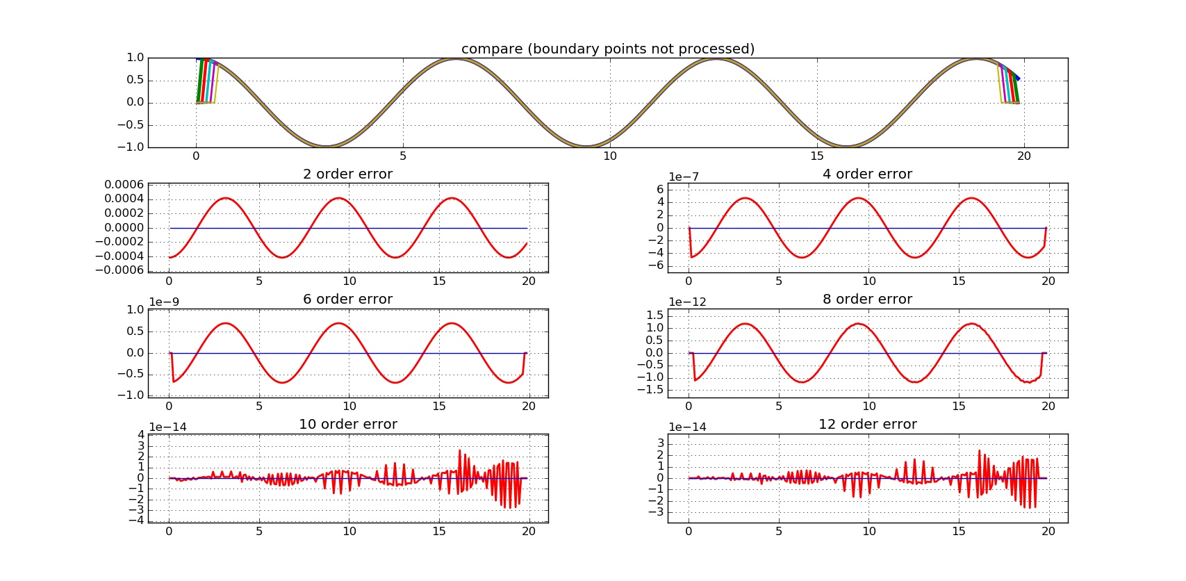
Examples

FD scheme corresponding to accuracy orders of 2,4,6,8,10,12 are implemented to $f(x) = sin(x)$, their FD results are ploted versus theoretical first order derivative of $f’(x) = cos(x)$, as well as their error.