Ray Tracing (2) Pseudo Bending Method

This post is about the pseudo bending method provided by Junho Um and Clifford Thurber. Test and codes are provided.

Intro

The key point of bending method is ray path calibration, which could be calculated according to $\eqref{rt1}$.

$$\begin{eqnarray} \frac{d^2x_i}{ds^2} = \frac{1}{c} ( -\frac{dc}{dx_i} + \frac{dc}{ds}\frac{dx_i}{ds} ) \label{rt1}\\ % T = \int_s \frac{1}{c}ds \label{rt2} \end{eqnarray}$$

In $\eqref{rt1}$, the left side is the ray path curvature, while the right side states the velocity gradient component normal to the ray path. This ray path curvature direction gives the calibration direction for each points:

$$\begin{eqnarray} \vec{n} = \nabla c - \frac{\vec{dx}}{|\vec{dx}|^2}\nabla c \cdot \vec{dx} \label{cur} \end{eqnarray}$$

The amount of calibration $R_c$ is obtained by minimizing the travel time.

Computation

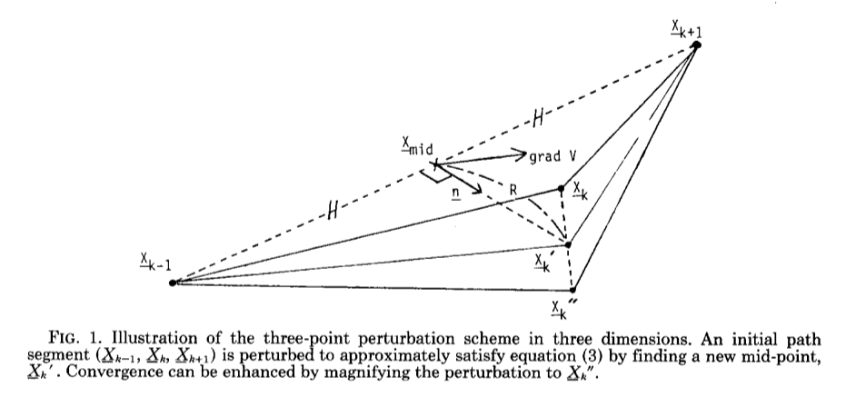
Discretize the seismic ray and analyze a segment of it:

The travel time for discretized ray path is:

$$\begin{eqnarray} T = \sum_{k=2}^{N} |\vec{X_k} - \vec{X_{k-1}}| \frac{c_k+c_{k-1}}{2} \end{eqnarray}$$

According to $\eqref{cur}$, the curvature direction for segment ($X{k-1}X{k+1}$) should be:

$$\begin{eqnarray} \vec{n} & = & \nabla c - \frac{\vec{X}_{k+1}- \vec{X}_{k-1}} {|\vec{X}_{k+1}- \vec{X}_{k-1}|^2}\nabla c \cdot (\vec{X}_{k+1}- \vec{X}_{k-1}) \label{e1} \end{eqnarray}$$

After having the curvature direction, a initial point is required. The mid-point is choosed, and the ideal point is $X_k’$.

Calibration amount is obtained by minimizing the travel-time of segment $X{k-1} \rightarrow X_k’ \rightarrow X{k+1}$.

$$\begin{eqnarray} R_c & = & -\frac{c_a c_{mid} + 1}{4c_a \vec{n}_0 \cdot \nabla c_{mid}} + \sqrt{ \Big( \frac{c_a c_{mid}+1}{4c_a \vec{n}_0 \cdot \nabla c_mid} \Big) + \frac{ |\vec{X}_{k+1} - \vec{X}_{mid}|^2}{ 2c_a c_{mid} } } \label{e2} \\ c_a & = & \frac{1}{2} \Big( \frac{1}{c_{k-1}} + \frac{1}{c_{k+1}} \Big) \\ \vec{n}_0 & = & \frac{ \vec{n} }{|\vec{n}|} \end{eqnarray}$$

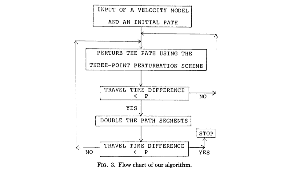
For each points of the seismic ray, apply $\eqref{e1}$ and $\eqref{e2}$ to acquire the new point. Repeat this procedure until the traveltime converges.

Moreover, more ray path control points are require for traveltime convergence. Um and Thurber provides a flow chart:

Codes & Test

1D constant gradient model

For one-dimensional constant velocity gradient model, the analytic ray path is an arc, the red line presented bellow. Ray paths of iteration are presented in black lines, which finally converge to the analytic ray path.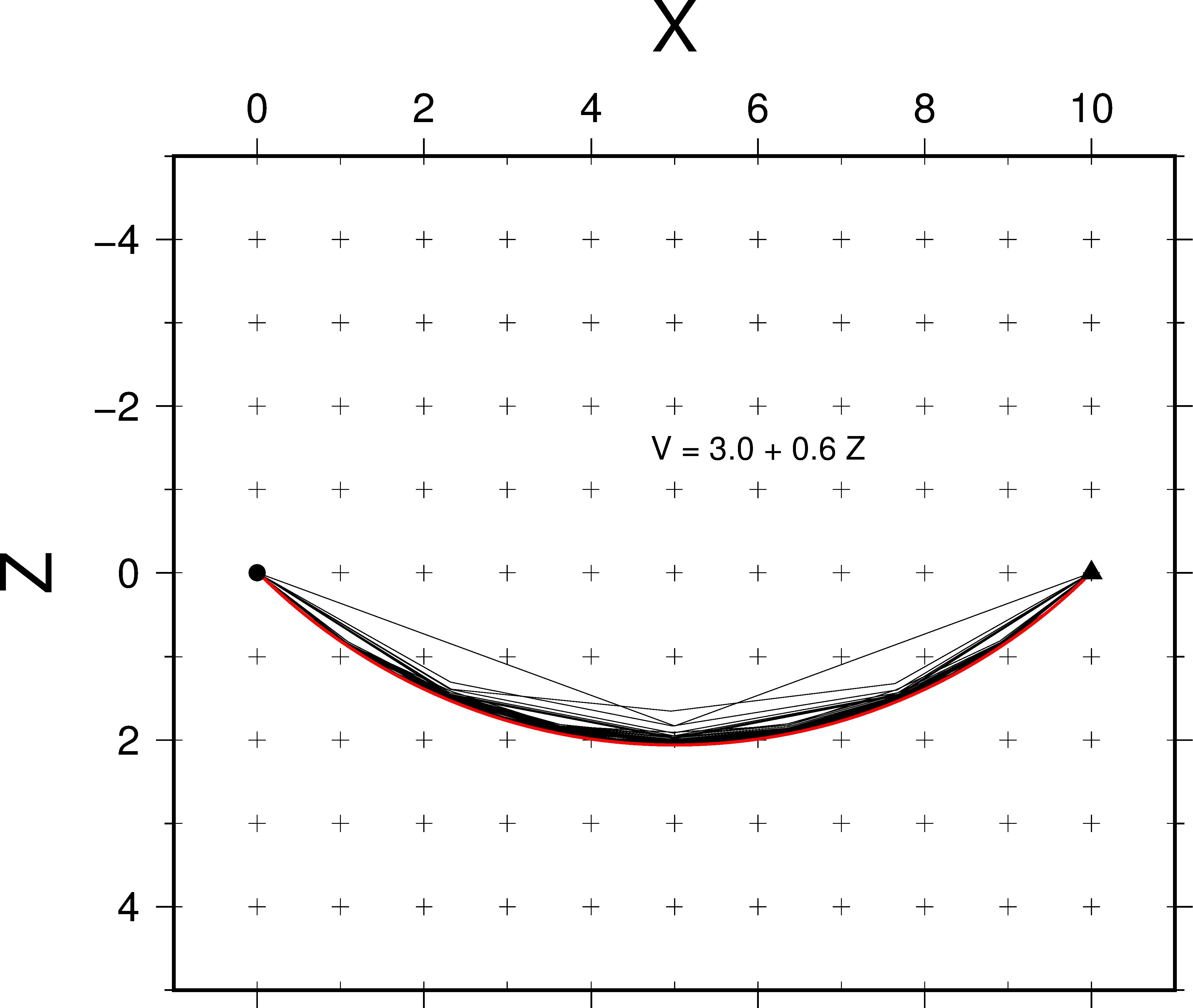

Codes

codes

bash> make
bash> ./main > path.dat
bash> ./plot.sh # "path.jpg" is the image of raypath
bash>

Reference

Um, J.,C.H. Thurber, A fast algorithm for two-point seismic ray tracing. Bull Seismol Soc Am.Bulletin of the Seismological Society of America, 1987. 77(3).